Choice [Micro Economics]

Micro Economics 

- Chapter 5. Choice

In this time we discuss about consumer theory and rational choice in economics. The lecture begins by reviewing previous concepts such as the budget constraint, preferences, and indifference curves. The main focus is on finding the optimal choice or most preferred affordable bundle for a consumer, subject to their budget constraint and preferences. The lecture discusses two types of solutions: interior solutions where both goods are consumed, and corner solutions where at least one good is not consumed. Various utility functions are explored, including Cobb-Douglas, perfect substitutes, perfect complements, and quasi-linear preferences. The lecture derives the conditions for optimal choice, such as exhausting the budget constraint and the tangency condition (where the slope of the indifference curve equals the slope of the budget constraint). Analytical solutions are provided for different utility functions, and graphical representations are used to illustrate the concepts. The lecture also addresses cases where the tangency condition may not hold or be sufficient for optimality. Overall, the lecture aims to equip students with the tools to analyze consumer behavior and find optimal choices under different preference structures and budget constraints.

Overview

1. Interior Solutions 

This time discusses interior solutions, where both goods are consumed with positive quantities at the optimal choice. The conditions for an interior solution are presented: exhausting the budget constraint and satisfying the tangency condition (where the slope of the indifference curve equals the slope of the budget constraint). The lecture derives the analytical solution for the Cobb-Douglas utility function and provides graphical representations to illustrate the concepts.

2. Corner Solutions 

This time explores corner solutions, where at least one good is not consumed at the optimal choice. Examples include perfect substitutes (where the consumer buys only the cheaper good), perfect complements (where the consumer buys goods in fixed proportions), and non-convex preferences. The lecture discusses the conditions for corner solutions and provides analytical solutions for specific utility functions.

3. Tangency Condition and Optimality 

This time discusses the role of the tangency condition in determining optimal choices. It is shown that the tangency condition is not always necessary or sufficient for optimality, and examples are provided where the tangency condition does not hold or does not define a unique optimum. The lecture clarifies the conditions under which the tangency condition is necessary and sufficient for optimality, such as continuous and strictly convex preferences.

3. Conclusion and Problem Set 

This time concludes by summarizing the conditions for finding the optimal consumer choice for rational consumers with strictly convex preferences. The solution involves solving a system of equations derived from the budget constraint and the tangency condition. The lecture recommends solving practice problems from the problem set to reinforce the concepts covered in the lecture.

Economic Rationality

Today we're gonna continue with the choice so it will be mainly a rational choice as we assume our decision maker is rational and able to choose what is best among all the alternatives that are affordable. 

The principal behavioral postulate is that a decisionmaker chooses its most preferred alternative from those available to it. & The available choices constitute the choice set.

We said earlier that the economic model of consumer choice is that people choose the best bundle they can afford. We can now rephrase this in terms that sound more professional by saying that “consumers choose the most preferred bundle from their budget sets.”

BC is defined as BC(p₁,p₂,m). Consumer's problem is to maximize U(x₁,x₂), it is objective. The choice variables x₁, x₂ can affect U, meanwhile BC has constant trait.

5.1 Optimal Choice

A typical case is illustrated in Figure 5.1. Here we have drawn the budget set and several of the consumer’s indifference curves on the same diagram. We want to find the bundle in the budget set that is on the highest indif- ference curve. Since preferences are well-behaved, so that more is preferred to less, we can restrict our attention to bundles of goods that lie on the budget line and not worry about those beneath the budget line.

The choice (x₁ , x₂ ) is an optimal choice for the consumer. The set of bundles that she prefers to (x₁ , x₂) the set of bundles above her indifference curve doesn’t intersect the bundles she can afford the bundles beneath her budget line. Thus the bundle (x₁ , x₂) is the best bundle that the consumer can afford.

Black line on upon Figure5.1 can be called Rational Constrained Choice (= Budget line).

In the Tangency condition, degree of point(x₁*, x₂*) is bP₁/aP₂

The Blue point of which exactly same point of Utility function & Rational constrained Choice line means "The most preferred of the affordable bundles. So, The Point (x₁*, x₂*) means most Affordable bundle.

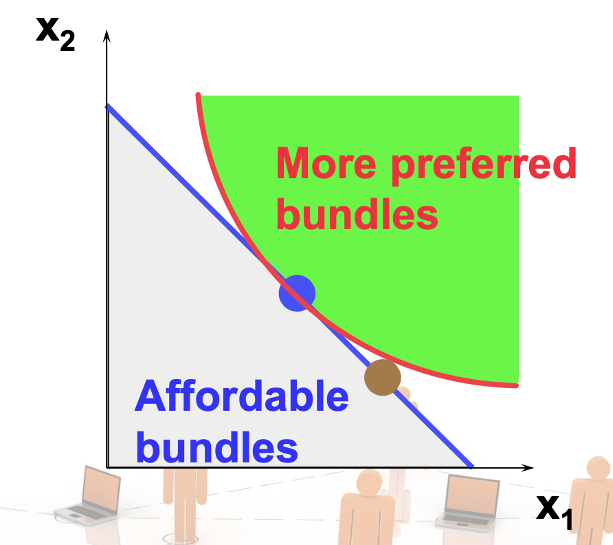
The most preferred affordable bundle is called the consumer’s Ordinary Demand at the given prices and budget.
Ordinary demands will be denoted by x₁*(p₁,p₂,m) & x₂*(p₁,p₂,m).
The (p₁,p₂,m) is BC. That means Budget Constraint.

**exhausts : 소진하다.

(x₁*,x₂*) is interior. (x₁*,x₂*) satisfies two conditions:

Case. a) (x₁*,x₂*) exhausts the budget ; p₁x₁* + p₂x₂* = m.
Case. b) Tangency Condition: The slope of the indifference curve at (x₁*,x₂*) equals the slope of the budget constraint.
[= the slope of the budget constraint, - p₁/p₂, and the slope of the indifference curve containing (x₁*,x₂*) are equal at (x₁*,x₂*)]

5.2 Consumer Demand

The optimal choice of goods 1 and 2 at some set of prices and income is called the consumer’s demanded bundle. In general when prices and income change, the consumer’s optimal choice will change. The demand function is the function that relates the optimal choice—the quantities demanded—to the different values of prices and incomes.

We will write the demand functions as depending on both prices and income: x1(p1, p2, m) and x2(p1, p2, m). For each different set of prices and income, there will be a different combination of goods that is the optimal choice of the consumer. Different preferences will lead to different demand functions; we’ll see some examples shortly. Our major goal in the next few chapters is to study the behavior of these demand functions—how the optimal choices change as prices and income change.

◆ How can this information be used to locate (x₁*,x₂*) for given p₁, p₂ and m?

MRS (= Marginal rate of substitution) : means preference about product x₁ upon x₂. 
Meaning x₁ is more prefers (a/b) times more than x₂

if A : MRS < p₁ / p₂
Then, that means MRS is more flatten than  p₁ / p₂
just willing to substitute a small amount of good 2 for good 1.

( MRS₁ or ₂ = - MU₁ / MU₂ )

Computing Ordinary Demands - a Cobb-Douglas Ex.

: Suppose that the consumer has Cobb- Douglas preferences

U(x₁,x₂)=x₁ª,x₂ᵇ

then, MRS = dx₂ / dx₁ => - ax₂ / bx₁ 

at (x₁*,x₂*) Tangency: MRS = - p₁ / p₂

x₂* = (a / b)(p₁ / p₂) x₁*

also (x₁*,x₂*) also exhausts the budget so p₁x₁* + p₂x₂* = m

So now we know that

(A) x₂* = (a / b)(p₁ / p₂) x₁*

(B) p₁x₁* + p₂x₂* = m

(이제 B에 A의 x₂*를 대입substitude한다)

Then get, p₁x₁* + p₂ (a / b)(p₁ / p₂) x₁* = m. /// ...  x₁* = am / (a+b)p₁

So we have discovered that the most preferred affordable bundle for a consumer with Cobb-Douglas preferences

U(x₁,x₂)=x₁ª,x₂ᵇ is

(x₁*,x₂*) = [ am / (a+b)p₁ , am / (a+b)p₂ ]

5.3 Some Examples

Let us apply the model of consumer choice we have developed to the exam- ples of preferences described in Chapter 3. The basic procedure will be the same for each example: plot 

Basic principle for solve problem :

When x₁* > 0 and x2* > 0 (interior solution) and (x₁*,x₂*) exhausts the budget, and preferences are strictly convex, the ordinary demands are obtained by solving:
    (a) p₁x₁*+p₂x₂*=m
    (b) the slopes of the budget constraint, - p₁/p₂, and of the indifference curve containing (x₁*,x₂*) are equal at (x₁*,x₂*).

Corner solution ( → Boundary optimum )

But what if x₁* = 0 or if x₂* = 0 ?

If either x₁* = 0 or x₂* = 0 then the ordinary demand (x₁*,x₂*) is at a corner solution to the problem of maximizing utility subject to a budget constraint.

We say that below represents a boundary optimum, while a case like upon represents an interior optimum.

++ the Perfect Substitutes(완전 대체재) Case & Quasi-linear Case has to be same kind of method within it.

when U(x₁,x₂) = x₁ + x₂ (=Perfect Substitutes function), the most preferred affordable bundle is (x₁*,x₂*)

where, 

(x₁*,x₂*) = ( y/p₁, 0 ) if p₁ < p₂

(x₁*,x₂*) = ( 0, y/p₂ ) if p₁ > p₂

+And, case in which MRS = -1 and have a condition Slope = -p1/p2 with p1 = p2.

In this case, All the bundles in the constraint are equally the most preferred affordable when p1 = p2.

Non-Convex Preferences Case ( → Boundary optimum )

※Caution: Notice that the “Tangency solution” is not the most preferred affordable bundle.

In this picture case, The most preferred affordable bundle is Boundary optimum.

Perfect Complements Case ( → interior optimum )

Optimal choice with perfect complements(완전 보완제)

If the goods are perfect complements, the quantities demanded will always lie on the diagonal since the optimal choice occurs where x₁ equals x₂.

※Caution: The Green point (x₁*,x₂*) is neither "MRS = - ∞" nor "MRS = 0", just MRS of (x₁*,x₂*) is undefined

:
(a) p₁x₁* + p₂x₂* = m
(b) x₂* = ax₁*

Substitution from (b) for x₂* in (a) gives p₁x₁* + p₂ax₁* = m
so which gives, x₁* = m / p₁ + ap₂ ; x₂* = am / p₁ + ap₂

Summary

1. The optimal choice of the consumer is that bundle in the consumer’s budget set that lies on the highest indifference curve.

2. Typically the optimal bundle will be characterized by the condition that the slope of the indifference curve (the MRS) will equal the slope of the budget line.

3. If we observe several consumption choices it may be possible to estimate a utility function that would generate that sort of choice behavior. Such a utility function can be used to predict future choices and to estimate the utility to consumers of new economic policies.

4. If everyone faces the same prices for the two goods, then everyone will have the same marginal rate of substitution, and will thus be willing to trade off the two goods in the same way.

[Reference]

[1] Hal R. Varian - Intermediate Microeconomics_ A Modern Approach, 8th Edition  -W.W. Norton & Co. (2010)